Using Torch FedAvg on MNIST dataset

This example illustrates the basic usage of SubstraFL, and proposes Federated Learning model training using the Federated Average strategy on the MNIST Dataset of handwritten digits using PyTorch. In this example, we work on 28x28 pixel sized grayscale images. The problem considered is a classification problem aiming to recognize the number written on each image..

SubstraFL can be used with any machine learning framework (PyTorch, Tensorflow, Scikit-Learn, etc). However a specific interface has been developed for PyTorch which makes writing PyTorch code simpler than with other frameworks. This example here uses the specific PyTorch interface.

This example does not use a deployed platform of Substra and run in local mode.

Requirements:

• To run this example locally, please make sure to download and unzip the assets needed to run it in the same directory as used this example:

  assets required to run this example

  Please ensure to have all the libraries installed. A requirements.txt file is included in the zip file, where you can run the command: pip install -r requirements.txt to install them.

• Substra and SubstraFL should already be installed. If not follow the instructions described here: Installation

Setup

We work with three different organizations. Two organizations provide a dataset, and a third one provides the algorithm and register the machine learning tasks.

This example runs in local mode, simulating a federated learning experiment.

In the following code cell, we define the different organizations needed for our FL experiment.

from substra import Client

N_CLIENTS = 3

# Every computation will run in `subprocess` mode, where everything run locally in Python
# subprocesses.
# Ohers backend_types are:
# "docker" mode where computations run locally in docker containers
# "remote" mode where computations run remotely (you need to have deployed platform for that)
client_0 = Client(backend_type="subprocess")
client_1 = Client(backend_type="subprocess")
client_2 = Client(backend_type="subprocess")
# To run in remote mode you have to also use the function `Client.login(username, password)`

clients = {
    client_0.organization_info().organization_id: client_0,
    client_1.organization_info().organization_id: client_1,
    client_2.organization_info().organization_id: client_2,
}


# Store organization IDs
ORGS_ID = list(clients.keys())
ALGO_ORG_ID = ORGS_ID[0]  # Algo provider is defined as the first organization.
DATA_PROVIDER_ORGS_ID = ORGS_ID[1:]  # Data providers orgs are the two last organizations.

Data and metrics

Data preparation

This section downloads (if needed) the MNIST dataset using the torchvision library. It extracts the images from the raw files and locally creates two folders: one for each organization.

Each organization will have access to half the train data, and to half the test data (which corresponds to 30,000 images for training and 5,000 for testing each).

import pathlib
from torch_fedavg_assets.dataset.mnist_dataset import setup_mnist


# Create the temporary directory for generated data
(pathlib.Path.cwd() / "tmp").mkdir(exist_ok=True)
data_path = pathlib.Path.cwd() / "tmp" / "data_mnist"

setup_mnist(data_path, len(DATA_PROVIDER_ORGS_ID))

Out:

Downloading http://yann.lecun.com/exdb/mnist/train-images-idx3-ubyte.gz
Downloading http://yann.lecun.com/exdb/mnist/train-images-idx3-ubyte.gz to /home/docs/checkouts/readthedocs.org/user_builds/owkin-substra-documentation/checkouts/0.23.1/substrafl_examples/get_started/tmp/data_mnist/MNIST/raw/train-images-idx3-ubyte.gz

  0%|          | 0/9912422 [00:00<?, ?it/s]
  2%|2         | 231424/9912422 [00:00<00:04, 2298040.92it/s]
 14%|#4        | 1394688/9912422 [00:00<00:01, 7757343.07it/s]
 54%|#####3    | 5324800/9912422 [00:00<00:00, 22122236.48it/s]
 99%|#########9| 9849856/9912422 [00:00<00:00, 30490892.86it/s]
9913344it [00:00, 24295126.49it/s]
Extracting /home/docs/checkouts/readthedocs.org/user_builds/owkin-substra-documentation/checkouts/0.23.1/substrafl_examples/get_started/tmp/data_mnist/MNIST/raw/train-images-idx3-ubyte.gz to /home/docs/checkouts/readthedocs.org/user_builds/owkin-substra-documentation/checkouts/0.23.1/substrafl_examples/get_started/tmp/data_mnist/MNIST/raw

Downloading http://yann.lecun.com/exdb/mnist/train-labels-idx1-ubyte.gz
Downloading http://yann.lecun.com/exdb/mnist/train-labels-idx1-ubyte.gz to /home/docs/checkouts/readthedocs.org/user_builds/owkin-substra-documentation/checkouts/0.23.1/substrafl_examples/get_started/tmp/data_mnist/MNIST/raw/train-labels-idx1-ubyte.gz

  0%|          | 0/28881 [00:00<?, ?it/s]
29696it [00:00, 13392908.77it/s]
Extracting /home/docs/checkouts/readthedocs.org/user_builds/owkin-substra-documentation/checkouts/0.23.1/substrafl_examples/get_started/tmp/data_mnist/MNIST/raw/train-labels-idx1-ubyte.gz to /home/docs/checkouts/readthedocs.org/user_builds/owkin-substra-documentation/checkouts/0.23.1/substrafl_examples/get_started/tmp/data_mnist/MNIST/raw

Downloading http://yann.lecun.com/exdb/mnist/t10k-images-idx3-ubyte.gz
Downloading http://yann.lecun.com/exdb/mnist/t10k-images-idx3-ubyte.gz to /home/docs/checkouts/readthedocs.org/user_builds/owkin-substra-documentation/checkouts/0.23.1/substrafl_examples/get_started/tmp/data_mnist/MNIST/raw/t10k-images-idx3-ubyte.gz

  0%|          | 0/1648877 [00:00<?, ?it/s]
 21%|##        | 339968/1648877 [00:00<00:00, 3397569.03it/s]
1649664it [00:00, 9941768.22it/s]
Extracting /home/docs/checkouts/readthedocs.org/user_builds/owkin-substra-documentation/checkouts/0.23.1/substrafl_examples/get_started/tmp/data_mnist/MNIST/raw/t10k-images-idx3-ubyte.gz to /home/docs/checkouts/readthedocs.org/user_builds/owkin-substra-documentation/checkouts/0.23.1/substrafl_examples/get_started/tmp/data_mnist/MNIST/raw

Downloading http://yann.lecun.com/exdb/mnist/t10k-labels-idx1-ubyte.gz
Downloading http://yann.lecun.com/exdb/mnist/t10k-labels-idx1-ubyte.gz to /home/docs/checkouts/readthedocs.org/user_builds/owkin-substra-documentation/checkouts/0.23.1/substrafl_examples/get_started/tmp/data_mnist/MNIST/raw/t10k-labels-idx1-ubyte.gz

  0%|          | 0/4542 [00:00<?, ?it/s]
5120it [00:00, 28330918.84it/s]
Extracting /home/docs/checkouts/readthedocs.org/user_builds/owkin-substra-documentation/checkouts/0.23.1/substrafl_examples/get_started/tmp/data_mnist/MNIST/raw/t10k-labels-idx1-ubyte.gz to /home/docs/checkouts/readthedocs.org/user_builds/owkin-substra-documentation/checkouts/0.23.1/substrafl_examples/get_started/tmp/data_mnist/MNIST/raw

Dataset registration

A Dataset is composed of an opener, which is a Python script that can load the data from the files in memory and a description markdown file. The Dataset object itself does not contain the data. The proper asset that contains the data is the datasample asset.

A datasample contains a local path to the data. A datasample can be linked to a dataset in order to add data to a dataset.

Data privacy is a key concept for Federated Learning experiments. That is why we set Permissions for each Assets to define which organization can use them.

Note that metadata, for instance: assets’ creation date, assets owner, are visible by all the organizations of a network.

from substra.sdk.schemas import DatasetSpec
from substra.sdk.schemas import Permissions
from substra.sdk.schemas import DataSampleSpec

assets_directory = pathlib.Path.cwd() / "torch_fedavg_assets"
dataset_keys = {}
train_datasample_keys = {}
test_datasample_keys = {}

for i, org_id in enumerate(DATA_PROVIDER_ORGS_ID):

    client = clients[org_id]

    permissions_dataset = Permissions(public=False, authorized_ids=[ALGO_ORG_ID])

    # DatasetSpec is the specification of a dataset. It makes sure every field
    # is well defined, and that our dataset is ready to be registered.
    # The real dataset object is created in the add_dataset method.

    dataset = DatasetSpec(
        name="MNIST",
        type="npy",
        data_opener=assets_directory / "dataset" / "mnist_opener.py",
        description=assets_directory / "dataset" / "description.md",
        permissions=permissions_dataset,
        logs_permission=permissions_dataset,
    )
    dataset_keys[org_id] = client.add_dataset(dataset)
    assert dataset_keys[org_id], "Missing dataset key"

    # Add the training data on each organization.
    data_sample = DataSampleSpec(
        data_manager_keys=[dataset_keys[org_id]],
        test_only=False,
        path=data_path / f"org_{i+1}" / "train",
    )
    train_datasample_keys[org_id] = client.add_data_sample(data_sample)

    # Add the testing data on each organization.
    data_sample = DataSampleSpec(
        data_manager_keys=[dataset_keys[org_id]],
        test_only=True,
        path=data_path / f"org_{i+1}" / "test",
    )
    test_datasample_keys[org_id] = client.add_data_sample(data_sample)

Metric registration

A metric is a function used to compute the score of predictions on one or several datasamples.

To add a metric, you need to define a function that computes and return a performance from the datasamples (as returned by the opener) and the predictions_path (to be loaded within the function).

When using a Torch SubstraFL algorithm, the predictions are saved in the predict function under the numpy format so that you can simply load them using np.load.

After defining the metrics dependencies and permissions, we use the add_metric function to register the metric. This metric will be used on the test datasamples to evaluate the model performances.

from sklearn.metrics import accuracy_score
import numpy as np

from substrafl.dependency import Dependency
from substrafl.remote.register import add_metric

permissions_metric = Permissions(public=False, authorized_ids=[ALGO_ORG_ID] + DATA_PROVIDER_ORGS_ID)

# The Dependency object is instantiated in order to install the right libraries in
# the Python environment of each organization.
metric_deps = Dependency(pypi_dependencies=["numpy==1.23.1", "scikit-learn==1.1.1"])


def accuracy(datasamples, predictions_path):
    y_true = datasamples["labels"]
    y_pred = np.load(predictions_path)

    return accuracy_score(y_true, np.argmax(y_pred, axis=1))


metric_key = add_metric(
    client=clients[ALGO_ORG_ID],
    metric_function=accuracy,
    permissions=permissions_metric,
    dependencies=metric_deps,
)

Specify the machine learning components

This section uses the PyTorch based SubstraFL API to simplify the machine learning components definition. However, SubstraFL is compatible with any machine learning framework.

In this section, you will:

• register a model and its dependencies

• specify the federated learning strategy

• specify the organizations where to train and where to aggregate

• specify the organizations where to test the models

• actually run the computations

Model definition

We choose to use a classic torch CNN as the model to train. The model structure is defined by the user independently of SubstraFL.

import torch
from torch import nn
import torch.nn.functional as F

seed = 42
torch.manual_seed(seed)


class CNN(nn.Module):
    def __init__(self):
        super(CNN, self).__init__()
        self.conv1 = nn.Conv2d(1, 32, kernel_size=5)
        self.conv2 = nn.Conv2d(32, 32, kernel_size=5)
        self.conv3 = nn.Conv2d(32, 64, kernel_size=5)
        self.fc1 = nn.Linear(3 * 3 * 64, 256)
        self.fc2 = nn.Linear(256, 10)

    def forward(self, x, eval=False):
        x = F.relu(self.conv1(x))
        x = F.relu(F.max_pool2d(self.conv2(x), 2))
        x = F.dropout(x, p=0.5, training=not eval)
        x = F.relu(F.max_pool2d(self.conv3(x), 2))
        x = F.dropout(x, p=0.5, training=not eval)
        x = x.view(-1, 3 * 3 * 64)
        x = F.relu(self.fc1(x))
        x = F.dropout(x, p=0.5, training=not eval)
        x = self.fc2(x)
        return F.log_softmax(x, dim=1)


model = CNN()
optimizer = torch.optim.Adam(model.parameters(), lr=0.001)
criterion = torch.nn.CrossEntropyLoss()

Specifying on how much data to train

To specify on how much data to train at each round, we use the index_generator object. We specify the batch size and the number of batches to consider for each round (called num_updates). See Index Generator for more details.

from substrafl.index_generator import NpIndexGenerator

# Number of model update between each FL strategy aggregation.
NUM_UPDATES = 100

# Number of samples per update.
BATCH_SIZE = 32

index_generator = NpIndexGenerator(
    batch_size=BATCH_SIZE,
    num_updates=NUM_UPDATES,
)

Torch Dataset definition

This torch Dataset is used to preprocess the data using the __getitem__ function.

This torch Dataset needs to have a specific __init__ signature, that must contain (self, datasamples, is_inference).

The __getitem__ function is expected to return (inputs, outputs) if is_inference is False, else only the inputs. This behavior can be changed by re-writing the _local_train or predict methods.

class TorchDataset(torch.utils.data.Dataset):
    def __init__(self, datasamples, is_inference: bool):
        self.x = datasamples["images"]
        self.y = datasamples["labels"]
        self.is_inference = is_inference

    def __getitem__(self, idx):

        if self.is_inference:
            x = torch.FloatTensor(self.x[idx][None, ...]) / 255
            return x

        else:
            x = torch.FloatTensor(self.x[idx][None, ...]) / 255

            y = torch.tensor(self.y[idx]).type(torch.int64)
            y = F.one_hot(y, 10)
            y = y.type(torch.float32)

            return x, y

    def __len__(self):
        return len(self.x)

SubstraFL algo definition

A SubstraFL Algo gathers all the elements that we defined that run locally in each organization. This is the only SubstraFL object that is framework specific (here PyTorch specific).

The TorchDataset is passed as a class to the Torch algorithm. Indeed, this TorchDataset will be instantiated directly on the data provider organization.

from substrafl.algorithms.pytorch import TorchFedAvgAlgo


class MyAlgo(TorchFedAvgAlgo):
    def __init__(self):
        super().__init__(
            model=model,
            criterion=criterion,
            optimizer=optimizer,
            index_generator=index_generator,
            dataset=TorchDataset,
            seed=seed,
        )

Federated Learning strategies

A FL strategy specifies how to train a model on distributed data. The most well known strategy is the Federated Averaging strategy: train locally a model on every organization, then aggregate the weight updates from every organization, and then apply locally at each organization the averaged updates.

from substrafl.strategies import FedAvg

strategy = FedAvg()

Where to train where to aggregate

We specify on which data we want to train our model, using the TrainDataNode objets. Here we train on the two datasets that we have registered earlier.

The AggregationNode specifies the organization on which the aggregation operation will be computed.

from substrafl.nodes import TrainDataNode
from substrafl.nodes import AggregationNode


aggregation_node = AggregationNode(ALGO_ORG_ID)

train_data_nodes = list()

for org_id in DATA_PROVIDER_ORGS_ID:

    # Create the Train Data Node (or training task) and save it in a list
    train_data_node = TrainDataNode(
        organization_id=org_id,
        data_manager_key=dataset_keys[org_id],
        data_sample_keys=[train_datasample_keys[org_id]],
    )
    train_data_nodes.append(train_data_node)

Where and when to test

With the same logic as the train nodes, we create TestDataNode to specify on which data we want to test our model.

The Evaluation Strategy defines where and at which frequency we evaluate the model, using the given metric(s) that you registered in a previous section.

from substrafl.nodes import TestDataNode
from substrafl.evaluation_strategy import EvaluationStrategy


test_data_nodes = list()

for org_id in DATA_PROVIDER_ORGS_ID:

    # Create the Test Data Node (or testing task) and save it in a list
    test_data_node = TestDataNode(
        organization_id=org_id,
        data_manager_key=dataset_keys[org_id],
        test_data_sample_keys=[test_datasample_keys[org_id]],
        metric_keys=[metric_key],
    )
    test_data_nodes.append(test_data_node)

# Test at the end of every round
my_eval_strategy = EvaluationStrategy(test_data_nodes=test_data_nodes, rounds=1)

Running the experiment

We now have all the necessary objects to launch our experiment. Please see a summary below of all the objects we created so far:

• A Client to add or retrieve the assets of our experiment, using their keys to identify them.

• An Torch algorithm to define the training parameters (optimizer, train function, predict function, etc…).

• A Federated Strategy, to specify how to train the model on distributed data.

• Train data nodes to indicate on which data to train.

• An Evaluation Strategy, to define where and at which frequency we evaluate the model.

• An AggregationNode, to specify the organization on which the aggregation operation will be computed.

• The number of rounds, a round being defined by a local training step followed by an aggregation operation.

• An experiment folder to save a summary of the operation made.

• The Dependency to define the libraries on which the experiment needs to run.

from substrafl.experiment import execute_experiment

# A round is defined by a local training step followed by an aggregation operation
NUM_ROUNDS = 3

# The Dependency object is instantiated in order to install the right libraries in
# the Python environment of each organization.
algo_deps = Dependency(pypi_dependencies=["numpy==1.23.1", "torch==1.11.0"])

compute_plan = execute_experiment(
    client=clients[ALGO_ORG_ID],
    algo=MyAlgo(),
    strategy=strategy,
    train_data_nodes=train_data_nodes,
    evaluation_strategy=my_eval_strategy,
    aggregation_node=aggregation_node,
    num_rounds=NUM_ROUNDS,
    experiment_folder=str(pathlib.Path.cwd() / "tmp" / "experiment_summaries"),
    dependencies=algo_deps,
)

Out:

Compute plan progress:   0%|          | 0/27 [00:00<?, ?it/s]/home/docs/checkouts/readthedocs.org/user_builds/owkin-substra-documentation/checkouts/0.23.1/docs/src/substra/substra/sdk/backends/local/backend.py:599: UserWarning: `transient=True` is ignored in local mode
  warnings.warn("`transient=True` is ignored in local mode")

Compute plan progress:   4%|3         | 1/27 [00:04<02:09,  4.97s/it]
Compute plan progress:   7%|7         | 2/27 [00:09<02:01,  4.85s/it]
Compute plan progress:  11%|#1        | 3/27 [00:13<01:42,  4.26s/it]
Compute plan progress:  15%|#4        | 4/27 [00:13<01:03,  2.75s/it]
Compute plan progress:  19%|#8        | 5/27 [00:17<01:06,  3.04s/it]
Compute plan progress:  22%|##2       | 6/27 [00:22<01:18,  3.72s/it]
Compute plan progress:  26%|##5       | 7/27 [00:27<01:22,  4.10s/it]
Compute plan progress:  30%|##9       | 8/27 [00:28<00:58,  3.07s/it]
Compute plan progress:  33%|###3      | 9/27 [00:28<00:42,  2.38s/it]
Compute plan progress:  37%|###7      | 10/27 [00:32<00:46,  2.75s/it]
Compute plan progress:  41%|####      | 11/27 [00:32<00:32,  2.04s/it]
Compute plan progress:  44%|####4     | 12/27 [00:36<00:37,  2.48s/it]
Compute plan progress:  48%|####8     | 13/27 [00:41<00:44,  3.20s/it]
Compute plan progress:  52%|#####1    | 14/27 [00:45<00:47,  3.62s/it]
Compute plan progress:  56%|#####5    | 15/27 [00:46<00:33,  2.79s/it]
Compute plan progress:  59%|#####9    | 16/27 [00:47<00:24,  2.20s/it]
Compute plan progress:  63%|######2   | 17/27 [00:51<00:26,  2.60s/it]
Compute plan progress:  67%|######6   | 18/27 [00:51<00:17,  1.95s/it]
Compute plan progress:  70%|#######   | 19/27 [00:54<00:18,  2.28s/it]
Compute plan progress:  74%|#######4  | 20/27 [00:59<00:20,  2.95s/it]
Compute plan progress:  78%|#######7  | 21/27 [01:03<00:20,  3.50s/it]
Compute plan progress:  81%|########1 | 22/27 [01:04<00:13,  2.71s/it]
Compute plan progress:  85%|########5 | 23/27 [01:05<00:08,  2.15s/it]
Compute plan progress:  89%|########8 | 24/27 [01:09<00:07,  2.60s/it]
Compute plan progress:  93%|#########2| 25/27 [01:12<00:05,  2.86s/it]
Compute plan progress:  96%|#########6| 26/27 [01:13<00:02,  2.26s/it]
Compute plan progress: 100%|##########| 27/27 [01:14<00:00,  1.84s/it]
Compute plan progress: 100%|##########| 27/27 [01:14<00:00,  2.76s/it]

Explore the results

List results

import pandas as pd

performances_df = pd.DataFrame(client.get_performances(compute_plan.key).dict())
print("\nPerformance Table: \n")
print(performances_df[["worker", "round_idx", "performance"]])

Out:

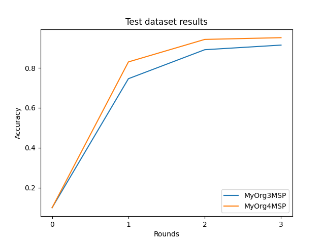
Performance Table:

      worker round_idx  performance
0  MyOrg3MSP         0       0.0990
1  MyOrg4MSP         0       0.0988
2  MyOrg3MSP         1       0.7458
3  MyOrg4MSP         1       0.8300
4  MyOrg3MSP         2       0.8912
5  MyOrg4MSP         2       0.9428
6  MyOrg3MSP         3       0.9144
7  MyOrg4MSP         3       0.9516

Plot results

import matplotlib.pyplot as plt

plt.title("Test dataset results")
plt.xlabel("Rounds")
plt.ylabel("Accuracy")

for id in DATA_PROVIDER_ORGS_ID:
    df = performances_df.query(f"worker == '{id}'")
    plt.plot(df["round_idx"], df["performance"], label=id)

plt.legend(loc="lower right")
plt.show()

Download a model

After the experiment, you might be interested in downloading your trained model. To do so, you will need the source code in order to reload your code architecture in memory. You have the option to choose the client and the round you are interested in downloading.

If round_idx is set to None, the last round will be selected by default.

from substrafl.model_loading import download_algo_files
from substrafl.model_loading import load_algo

client_to_dowload_from = DATA_PROVIDER_ORGS_ID[0]
round_idx = None

algo_files_folder = str(pathlib.Path.cwd() / "tmp" / "algo_files")

download_algo_files(
    client=clients[client_to_dowload_from],
    compute_plan_key=compute_plan.key,
    round_idx=round_idx,
    dest_folder=algo_files_folder,
)

model = load_algo(input_folder=algo_files_folder).model

print(model)

Out:

CNN(
  (conv1): Conv2d(1, 32, kernel_size=(5, 5), stride=(1, 1))
  (conv2): Conv2d(32, 32, kernel_size=(5, 5), stride=(1, 1))
  (conv3): Conv2d(32, 64, kernel_size=(5, 5), stride=(1, 1))
  (fc1): Linear(in_features=576, out_features=256, bias=True)
  (fc2): Linear(in_features=256, out_features=10, bias=True)
)